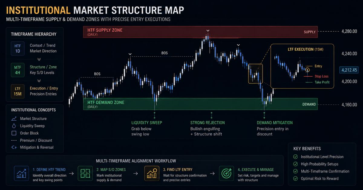
The structural dynamics of modern electronic financial markets are not governed by arbitrary retail geometric lines, trend channels, or mathematical lagging indicator cross-overs. Instead, the global order book moves systematically based on the mechanics of liquidity delivery, institutional order flow, and structural imbalances. To trade effectively alongside major market participants, a structural operator must look past localized market noise and learn to track institutional order blocks. This comprehensive guide outlines the foundational mechanics of Multi-Timeframe Supply and Demand Trading—commonly referred to within institutional spaces as Smart Money Concepts (SMC)—providing you with a robust, rules-based framework to identify, map, and execute high-expectancy setups across nested time horizons.
The Institutional Paradigm: Deconstructing Supply and Demand
To understand why conventional support and demand technical setups consistently trap retail traders, you must understand how institutional orders are fulfilled. Large entities, such as central banks, algorithmic sovereign funds, and tier-one investment firms, cannot simply click an execution trigger to buy thousands of lots without creating massive slippage. They require counterparty liquidity to match their massive transaction allocations.
Therefore, a true Demand Zone is not just a general area where price previously bounced; it is a highly specific footprint where a dominant participant deployed significant capital, creating a structural imbalance. When price moves away from these zones rapidly, it leaves behind unmitigated orders. Professional operators anticipate the eventual return to these resting orders.
Failing to respect this higher-timeframe macro environment frequently leads to catastrophic risk acceleration. If an operator executes a trade blindly into unmitigated macro imbalances without understanding the broader structure, they risk a rapid capital draw. This is the exact mechanical trap that explains how leverage can become your trading enemy when market makers aggressively hunt resting liquidity pools.
Anatomy of a Valid Structural Order Block
Not all candlesticks that precede an aggressive expansion qualify as high-probability supply or demand zones. To separate high-expectancy institutional zones from minor market noise, an order block must meet three strict structural criteria:
- Liquidity Capture (The Sweep): The institutional candlestick must actively sweep a previous minor swing high or low, absorbing the resting stop orders of retail breakout or trend participants before reversing direction.
- Displacement & Inefficiency: The subsequent exit from the zone must be highly aggressive, characterized by large, expanding candle bodies that construct an explicit Fair Value Gap (FVG) or structural market imbalance.
- Break of Structure (BOS): The expansion must successfully close beyond the opposing swing high or swing low on that specific timeframe, confirming a clean, undeniable shift in localized market dominance.
The Core Framework: Multi-Timeframe Structural Nesting
The true edge in supply and demand trading comes from combining multiple timeframes. Executing a trade based strictly on a single timeframe exposes an operator to localized noise. A clean M5 demand zone, for example, will easily fail if it rests within a massive H4 supply zone.
To trade with structural alignment, we employ a top-down nesting strategy using three distinct temporal layers:
- Macro Directional Filter (Daily/H4 Timeframe): We map the major swing structural legs, identify external liquidity pools, and draw our premium and discount supply and demand zones. This tells us our macro directional bias.
- Medium-Term Structural Bridge (H1/M15 Timeframe): We observe price as it approaches our macro zone, tracking internal market structure to ensure that mid-term order flow aligns with our intended macro direction.
- Micro Execution Engine (M5/M1 Timeframe): Once price reaches the high-timeframe zone, we drop down to our lowest execution horizon. We watch for a localized entry trigger—the initial shift in internal order flow known as a Change of Character (CHoCH). To master the granular mechanical differences between a standard structural trend continuation and an execution-level trend reversal, deep-dive into our explicit sub-system breakdown: Mastering Market Structure: What are BOS and CHoCH?.
⚡ Technical Analysis Synergy: Deploying sub-millisecond execution tools works best when you are aligned with institutional order flow. Master our top-down structural framework in Multi-Timeframe Analysis: How to Identify High-Probability Trends.
The Blueprint Components: Advanced Order Flow Sub-Systems
To fully scale this multi-timeframe framework into a rigid, quantitative trading enterprise, a structural operator cannot rely on vague zone drawings or general eye-balling techniques. The overarching matrix relies on two critical sub-components that manage execution precision and mathematical validity:
First, your boundary mapping must be fully mechanized. Instead of enveloping massive multi-candle clusters that inflate your capital exposure, you must isolate the core footprints of institutional mitigation. Our strict mechanical rule plots demand arrays explicitly from the first candle body down to the terminal lowest wick of that sequence. To learn the precise implementation parameters for both sides of the market book, read our specialized blueprint on Precision Zone Mapping: Mechanical Boundaries for Demand and Supply Order Blocks.
Second, a structural block is only as powerful as the displacement it delivers. To mathematically screen out low-expectancy market noise, every mapped zone must be vetted against localized price inefficiencies. Discovering an open three-candle void confirms that major algorithmic engines have left incomplete order books. Master how to systematically execute this filter by reading Validating Order Flow Inefficiencies: Using Fair Value Gaps (FVG) to Filter High-Probability Zones.
Advanced Structural Synergy Index
The table below demonstrates how structural operators evaluate multi-timeframe variables to categorize trade setups based on their probability of success:
| Macro H4 Array Context | M15 Internal Structure | M1 Execution Confirmation | Operational Priority Rating |
|---|---|---|---|
| Discount Demand Zone Tap | Bullish Break of Structure (BOS) | CHoCH + Micro FVG Mitigation | High (Full Structural Synergy) |
| Discount Demand Zone Tap | Bearish Internal Flow (Downtrend) | No Entry Signal / Liquidity Sweep Pending | Neutral (Patience Required) |
| Premium Supply Zone Tap | Bearish Break of Structure (BOS) | CHoCH + Micro Supply Mitigated | High (Pro-Trend Short Vector) |
| No High-Timeframe Array (Mid-Range) | Bullish Expansion | Micro CHoCH Observed | Low (High Inversion Trap Risk) |
Risk Mitigation Matrix for the Structural Operator
Nesting executions on lower charts like the M1 allows for highly asymmetric risk-to-reward profiles. However, it also introduces a key challenge: position sizing variance. Because your structural stop loss is tucked tightly behind a micro order block, your validation boundary could be as small as 3 to 5 pips.
Executing arbitrary lot sizes on these tight boundaries can cause severe drawdowns if a sequence of minor stop-outs occurs. To protect your equity curve, you must dynamically scale your lot allocations using precise quantitative calculators. For example, when trading precious metals, using a dedicated Gold Position Size Calculator ensures that your capital risk remains perfectly fixed regardless of shifting structural volatility.
Furthermore, for operators navigating funding evaluations or managing capital within precise proprietary firms, tracking cumulative portfolio exposure is critical. Utilizing a comprehensive Prop Firm Drawdown Calculator ensures that minor counter-trend sweeps do not accidentally violate your daily drawdown limits. If you have recently experienced performance degradation due to over-leveraging these micro-entries, we highly recommend following a systematic approach, such as the one outlined in the ultimate drawdown recovery guide, to realign your execution psychology and protect your account balance.
Conclusion: Developing a Systematic Edge
Transitioning to multi-timeframe supply and demand trading requires letting go of retail technical bias and adopting a purely structural perspective. By focusing on higher-timeframe order blocks, waiting for price to return to these zones, and using lower-timeframes exclusively to find refined, high-asymmetry entry points, you insulate your capital from market noise. Maintain rigorous risk parameters, protect your portfolio from volatility spikes, and let structural mechanics drive your long-term consistency.
Smart Money Concepts & Order Flow FAQ
How do you systematically differentiate between a valid structural break (BOS) and a liquidity sweep?
A valid Break of Structure (BOS) requires a definitive candle body closure beyond the established swing high or swing low on the tracking timeframe. Conversely, a liquidity sweep occurs when price breaches a structural level via a wick but fails to sustain momentum, closing back within the previous range to trap breakout participants before reversing.
Why do high-timeframe supply and demand zones override lower-timeframe structural patterns?
High-timeframe zones (such as H4, D1, or W1) represent the structural footprints of major institutional accumulation and distribution cycles. Lower-timeframe patterns within these zones are merely noise generated by localized order-matching mechanics; their primary purpose is providing refined entries into the macro structural order flow.
What is the mechanical relationship between an Imbalance (Fair Value Gap) and a valid demand zone?
An Imbalance or Fair Value Gap (FVG) indicates a highly aggressive market inefficiency where only one side of the order book was aggressively filled. A premium or discount demand zone accompanied by an immediate, clear FVG confirms institutional capital commitment, increasing the probability that price will return to mitigate that specific sector.
How does an operator manage capital exposure when trading volatile low-timeframe executions?
Operators must dynamically calibrate position sizes based on the absolute pip distance of the lower-timeframe structural stop loss. Since entering on an M1 or M5 confirmation yields tight validation boundaries, position sizes must expand or contract to keep capital risk fixed relative to the portfolio's absolute balance.
What is the primary operational failure vector when executing multi-timeframe supply and demand systems?
The primary operational failure vector is execution impatience, specifically entering trades on lower-timeframes before price has systematically reached a validated high-timeframe demand or supply array. This leads to getting caught in minor counter-trend liquidity sweeps and experiencing premature stop-outs.